Cell Foundations: The Single Cell Revolution 2

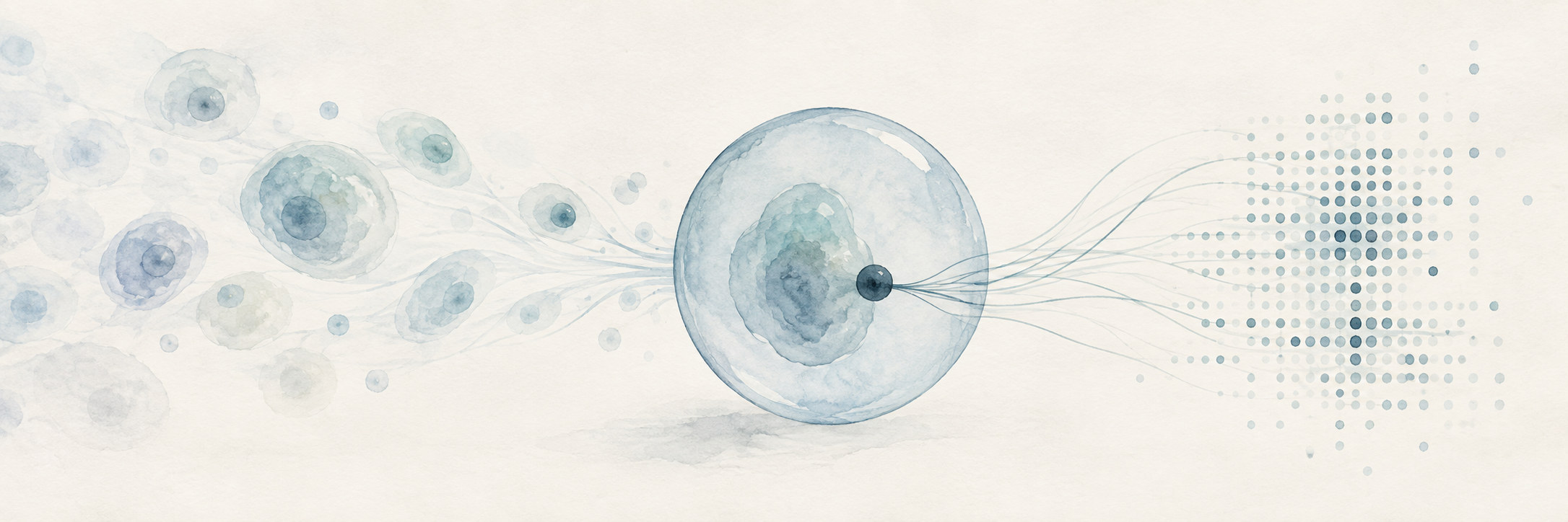
Part 2 - Drop-seq

Drop-seq is an innovation which allowed single-cell RNA sequencing to scale, building on established methods including cell dissociation, reverse transcription, PCR, microfluidics, molecular barcoding, and next-generation sequencing. Macosko and colleagues combined them so that RNA from thousands of cells could be processed together while preserving enough information to tie each captured molecule back to its cell of origin.^[1]

Before Drop-seq, one of the clearest ways to preserve that origin was to place one cell into each well of a plate. The well itself then preserved the cell's identity, but every cell remained a separate sample through the reactions which followed. Eric Chow explains how this meant only hundreds or perhaps a few thousand cells could be studied through a laborious amount of pipetting, labor, and cost, since each cell required its own miniature library preparation.^[2]

So Drop-seq replaced that persistent physical separation with what the authors called a "molecular memory." If we continue the factory model from Part One, the problem is like sending working recipes from thousands of factories into a single central mailroom. The recipe alone cannot reliably identify its source because several factories may use the same instructions, like how a car plant and an appliance factory might both contain work orders for the same standardized electric motor, bearing, or fastener. Drop-seq labels each captured recipe with a factory address before the order is sent.

In other words, the critical advance can be thought of as a bookkeeping. Thousands of cells could now share the same tubes, chemical reactions, sequencing library, and sequencing run because the origin of their RNA had been transferred from physical location into DNA sequence. From here, we can understand the process by following that address from the bead, through one droplet, and eventually into the final data table.

First, the address begins on a microscopic bead covered with DNA primers. Each primer is built from several short sequences with separate functions, including a common handle for later reactions, a cell barcode, a unique molecular identifier, and a tail of thymidines which can capture messenger RNA.^[1]

And every primer on one bead carries the same cell barcode, while different beads are intended to carry different barcodes. In the factory analogy, this is the factory address, although it is assigned by the experiment and has no relationship to the cell's location or biological identity. If one bead meets one cell, all messenger RNA captured by that bead receives the same artificial address.

Next, the unique molecular identifier (UMI), performs a different job by varying among primers on the same bead, so two messenger RNA molecules captured from one cell can receive the same cell barcode but different molecular identifiers. This is particularly clever because PCR will later make many copies of the resulting DNA. If fifty sequencing reads map to the same gene and carry the same cell barcode and UMI, the most likely explanation is that PCR copied one captured molecule fifty times, and only reads with different UMIs provide evidence for separate molecules of origin.^[3]

So the cell barcode identifies the factory, while the UMI provides something like a serial number for an individual recipe taken from that factory. This distinction is what eventually allows the experiment to estimate molecules instead of counting whichever PCR copies happened to become most abundant.

Finally, at the free end of every primer is oligo-dT, a sequence made from repeated thymidines which binds the poly(A) tail found on most mature protein-coding messenger RNA and acts as the molecular hook. It gives the bead one shared way to capture thousands of different messenger RNAs, although it also acts as a filter which defines what can enter the measurement. Ribosomal RNA and many other non-polyadenylated RNAs generally lack the required handle, but even compatible messenger RNA can still degrade or escape capture.

Next, separate streams carry cells and beads into a microfluidic device, where oil pinches the water-based mixture into droplets. In the useful case, one droplet contains one cell and one bead, and the droplet acts as a temporary sealed room small enough for the cell to be lysed and for its released messenger RNA to encounter the bead before material from other cells enters the same space.^[1][2]

Lysis means that the cell membrane is broken apart, after which the factory is demolished, its messenger RNA spills into the mailroom, and polyadenylated molecules bind to the oligo-dT hooks on the bead. Once that capture has occurred, the bead carries the information needed to preserve origin through the pooled steps which follow.

However, cells and beads enter the Drop-seq device randomly. In the original 2015 implementation, most droplets were therefore empty or contained only one of the required components, while a small fraction contained the useful combination of one cell and one bead. Loading more cells increases the number of productive droplets, but it also increases the probability that two cells enter together. Their RNA then receives one cell barcode and produces a combined profile which corresponds to neither original cell. This is called a doublet, while droplets with still more cells are called multiplets.^[2] While there are stastitical methods to correct for doublets and multiplets, these are tradeoffs which need to be considered.

In fact, Macosko and colleagues measured the extent of this tradeoff using mixtures of human and mouse cells. As cell concentration increased across the tested range, the estimated doublet rate rose from 0.36 percent to 11.3 percent, while processing speed increased from about 1,200 to about 10,000 cells per hour.^[1] So in this implementation, empty droplets were part of the accuracy strategy, since wasted capacity costs reagents while a doublet can manufacture a plausible cell in the data which never actually existed.

Next, in the original Drop-seq workflow, the droplets could be broken after messenger RNA had attached to the primers. The beads were collected and washed together, then reverse transcription occurred on the captured material.^[1] The droplet itself is only needed to keep each cell's RNA separate until the RNA binds to its barcoded bead. Once that happens, the barcode preserves the cell of origin, so the droplets can be broken and the beads pooled.

The reverse transcriptase uses each captured messenger RNA as a template to build complementary DNA, usually called cDNA. RNA is the short-lived working copy produced by the cell, while cDNA is a laboratory-made copy suitable for amplification and sequencing, and since the bead primer already contains the cell barcode and UMI, those labels become part of the resulting construct.^[1]

In other words, reverse transcription converts the biological RNA into DNA carrying known technical sequences, and PCR then produces enough copies of that DNA for the later reactions to work. Library preparation then breaks the amplified DNA into manageable fragments and adds adapters, which are standardized DNA connectors that allow the fragments to bind to and be read by a sequencing system.^[4][5]

However, PCR introduces its own distortion because different starting molecules can amplify at different rates. One cDNA may produce hundreds of descendants while another produces only a few, and this is where the UMI allows the analysis to collapse descendants carrying the same cell barcode, gene assignment, and molecular identifier back toward one captured molecule. But any messenger RNA lost before a primer supplied that identifier will be left out of the final data set.

Then, inside, say, an Illumina sequencer, adapter-bearing fragments bind to a glass flow cell and form local clusters of matching copies, creating a signal bright enough for the instrument to read. During repeated cycles, a fluorescently labeled DNA base is added, an image records its identity, and the process continues to recover a short sequence from each cluster.^[4][5]

One read recovers the cell barcode and UMI, answering where the captured molecule was assigned and which starting molecule it may represent. The paired read samples RNA-derived cDNA, providing a short excerpt which can be matched against a reference genome and gene annotation.^[1] In the same way a short quotation can identify a known book without requiring the entire text, a short cDNA sequence can often identify the gene which produced the messenger RNA.

However, the excerpt comes from near the 3-prime end where the poly(A) tail was captured. This makes Drop-seq effective for gene-level counting and usually leaves too little information to reconstruct which internal exons were joined into a particular transcript isoform. As discussed in Part One, this means alternative splicing is mostly lost. Full-length plate methods preserve more of that structure and detect more genes per cell, while droplet methods accept a shallower record in exchange for sampling many more cells.^[6]

After sequencing, the original cells have disappeared and millions of short reads remain. The computer assigns the RNA-derived sequence to a gene, groups reads by their cell barcode, and uses UMIs to reduce repeated PCR descendants to inferred captured molecules, producing a cell-by-gene count matrix. Each row represents an annotated gene, each column represents a barcode judged to contain a cell, and each entry estimates how many messenger RNA molecules from that gene survived the measurement chain.^[1]

However, even the column described as one cell requires judgment. For instance, some beads encounter ambient RNA released by damaged cells without ever sharing a droplet with an intact cell. The original analysis ranked barcodes by their total molecule counts and used the change in that distribution to separate likely cell-containing beads from the long background tail. In this way, a small real cell can fall toward the background, while an empty bead with enough ambient RNA can appear as a definitive measure.

And even after likely cells have been separated from the ambient background, each retained profile contains only a fraction of the cell's messenger RNA. Macosko and colleagues estimated this fraction by supplying synthetic RNA at known concentrations and measuring how much Drop-seq recovered. The system captured about 12.8 percent of those molecules, while a separate comparison using digital PCR across ten genes produced an average estimate of 10.7 percent.^[1]

This incompleteness also makes a zero reading ambiguous. The gene may have been inactive, or the cell may have been caught between transcriptional bursts, but its messenger RNA may also have existed and escaped capture. Missing every molecule becomes especially likely when a gene produces only a few copies of that molecule, which is one source of the dropout Kellis describes in single-cell data.^[3] The count matrix is therefore a partial sample of the cell's messenger RNA population, even when every computational step is performed perfectly.

What Drop-seq changed

The original Drop-seq design accepted less information from each cell in order to measure enough cells to reveal population structure. This is the same tradeoff Part One introduced, now shown explicitly in the mechanism of the method itself. The droplet creates the address, the UMI makes amplification partly correctable, the short cDNA read identifies a gene, and the pooled library makes the marginal preparation cost of another cell far smaller than maintaining another well through every reaction.

Macosko and colleagues' retina experiment showed what this exchange made possible. Researchers had already identified roughly 100 mouse retinal cell types through their shape, electrical behavior, and function, although fewer than half had a known molecular marker which could identify them directly. The authors wondered whether cells could instead be organized from their gene expression alone. When they compared RNA profiles from 44,808 retinal cells, five known neuronal classes emerged from the data, along with 39 smaller transcriptional populations.^[1]

However, the result was incomplete, since 39 transcriptional populations left many of the roughly 100 morphologically or functionally defined types unresolved. Its narrower value was that one experiment surveyed tens of thousands of cells and generated candidate molecular signatures which could be tested against populations previously distinguished through slower morphological or functional study. This provided evidence that the exchange of depth for scale could work, while the unresolved types also showed how much resolution had been lost.